A Hands-On Guide to Automatic Music Generation using RNN

Machine learning is now being used for many interesting applications in a variety of fields. Music generation is one of the interesting applications of machine learning. As music itself is sequential data, it can be modelled using a sequential machine learning model such as the recurrent neural network. This modelling can help in learning the music sequence and generating the sequence of music data. In this article, we are going to discuss how we can use neural networks, specifically recurrent neural networks for automatic music generation. The major points to be discussed in this article are listed below.

Table of Contents

1. Understanding a Music File
2. About Recurrent Neural Network (RNN)
3. Why Music File with RNN?
4. Implementation in Python

Understanding a Music File

In a programming context, we can consider music as data that can give many insightful results by processing it with various procedures. Before processing it, we are required to know what type of information a music file can consist of. First of all, a piece of very basic information about any audio or music file is that it can be made up of three parts:

• Pitch: It is a measure of the highness or lowness of the sound.
• Notes: There can be seven types of notes in a music file which can be expressed as A, B, C, D, E. F, AND G. 
• Octave: In music, we use the octave to explain the pitch range of any note. Like what is the measure of the highness of the note A in the music.  

The below image is a representation of the piano keyboard where we can use 88 keys and 7 octaves to make music from it.

Image source

We can use an example to explain the above-given terminology. Let’s say we need to talk about the comparison of sound from different keys of octaves, so the sound produced by the key B1(octave 1) will be lower than the sound produced by the B7 (octave 7). So this is how a music producer uses the pitch variation of different octaves and the sound of different nodes to produce some music out of a piano.

There are also various details like amplitude and frequencies that need to be known which are also a kind of information consisting of a music file. This information is used for defining the music file as sequential data. In this article, we are going to use the above-given information of music for processing it. A detailed explanation of the frequency and amplitude can be found here. Let’s start our next section of the article by introducing recurrent neural networks.        

About Recurrent Neural Network (RNN)

Before going into the implementation with RNN, let us discuss some basic facts of RNN( Recurrent Neural Network). In the family of neural networks, the RNN is a member of feedback neural networks (a subfamily of neural networks) with feedback connections. The ability to send information over time-steps makes the RNN different from the other members of the family of the neural network. When we talk about the working style of RNN, it considers sequential information as input and provides information in sequential form instead of accepting stable input and providing stable output. 

The output provided by the layers inside the networks re-enters into the layer as the input which helps in computing the value of the layer and by this process the network makes itself learn based on the current data and previous data together. Talking about the architecture of the basic RNN, we can say that an RNN consists of many copies of the neural network connected and working in a chain. 

Image source

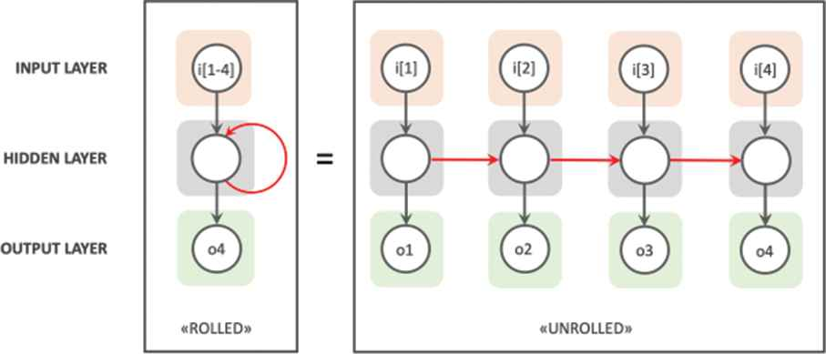
The above image can be considered as a representation of the architecture of RNN.

Why Music File with RNN?

As we have discussed the capabilities of the RNN are that it can work with sequential data as input and output. The audio data is also sequential data where it can be considered as a signal which has modulation with time similarly to the time series data where data points are collected in a  sequence with time values. Computer stores audio data in digital form of a series of 1’s and 0’s. Most of the time, the format for storing the data is pulse-code modulation by taking samples at a repeated rate. The Representation of the audio file can be done by the spectrograms. The spectrogram is made up of plotting frequency with time or amplitude with time. An example of a spectrogram is given below.

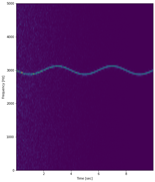
You can find a brief explanation of the spectrograms here. We are talking about the spectrogram just to know that the audio files are sequential data dependent on the sequences of some numeric values with time. Simply saying when a computer stores the audio data it stores the changes in the numeric values with time. The RNN and especially the LSTM models are well known for their performance in the field of sequence to sequence modelling.

Implementation

In this section of the article, we are going to see how we can generate musical notes using a simple RNN model. For this purpose, we will be using a library pretty_midi for datasets

Let’s start with the installation of pyfluidsynth and pretty_midi library.

Installing pyfluidsynth:

!sudo apt install -y fluidsynth

Output:

Installing pretty_midi:

!pip install pretty_midi

Output:

Importing Basic libraries:

import collections
import datetime
import fluidsynth
import glob
import numpy as np
import pathlib
import pandas as pd
import tensorflow as tf
from IPython import display
tf.random.set_seed(42)
np.random.seed(42)

For this implementation, we are going to use data from the maestro datasets where we have 1282 files of MIDI. we can get the data from this link. After downloading it, we are required to save the data in a directory from which we can extract the MIDI files.

From the maestro dataset, we can extract a MIDI file using the following lines of code.

sample_file = glob.glob(str(pathlib.Path('data/maestro-v2.0.0')/'**/*.mid*'))[1]
print(sample_file)

Output:

Here in the output, we can see that we have a file in the midi extension. Using this file, we can make an instance of the pretty_midi library.

import pretty_midi
file = pretty_midi.PrettyMIDI(sample_file)

Let’s play a file from the dataset. 

waveform = file.fluidsynth(fs=16000)
waveform_short = waveform[:30*16000]
display.Audio(waveform_short, rate=16000)

Here, we have chosen the sampling rate of 16000 for audio playback and we trimmed the file for 30 seconds. We can also know about the instruments used to make the music.

print('Number of instruments:', len(file.instruments))
print('Instrument name:', pretty_midi.program_to_instrument_name(file.instruments[0].program))

Output:

Now in the first section of the article, we have talked about the arrangement of notes, pitch and octave of the piano. Here we can see that the instrument used in the file is the piano. Let’s extract the notes from the music.

let’s check for the notes in the music

instrument = file.instruments[0]

for i, note in enumerate(instrument.notes[:15]):
  print(f'{i}: pitch={note.pitch}, note_name={pretty_midi.note_number_to_name(note.pitch)},'
        f' duration={note.end - note.start:.4f}')

Output:

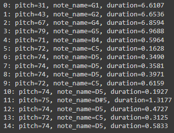
Here we can see the notes and pitch with the duration in the output. As we have discussed we are going to use this information in the process. We are required to make it available in Pandas DataFrame. 

Let’s extract the information.

def midi_to_df(files: str) -> pd.DataFrame:
  pm = pretty_midi.PrettyMIDI(files)
  instrument = pm.instruments[0]
  notes = collections.defaultdict(list)
  # Sort the notes by start time
  sorted_notes = sorted(instrument.notes, key=lambda note: note.start)
  prev_start = sorted_notes[0].start
  for note in sorted_notes:
    start = note.start
    end = note.end
    notes['pitch'].append(note.pitch)
    notes['start'].append(start)
    notes['end'].append(end)
    notes['step'].append(start - prev_start)
    notes['duration'].append(end - start)
    prev_start = start
  return pd.DataFrame({name: np.array(value) for name, value in notes.items()})
music_df = midi_to_df(sample_file)
music_df.head(10)

Output:

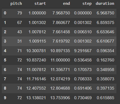
Here, the step shows the time elapsed from the previous note or start of the track. Let’s check the distribution of each note variable.

import seaborn as sns
import matplotlib.pyplot as plt
plt.figure(figsize=[15, 5])
plt.subplot(1, 3, 1)
sns.histplot(music_df, x="pitch", bins=20)
plt.figure(figsize=[15, 5])
plt.subplot(1, 3, 1)
sns.histplot(music_df, x="step", bins=20)
plt.figure(figsize=[15, 5])
plt.subplot(1, 3, 1)
sns.histplot(music_df, x="duratio", bins=20)

Output:

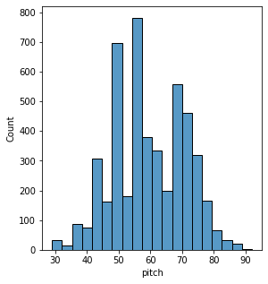
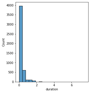
Our main objective in this article is to generate music automatically using an RNN model. For that, we are required to have a tensor on which the network can learn to predict. 

Let’s create a tensor. 

all_notes = []
for f in filenames[:5]:
  notes = midi_to_df(f)
  all_notes.append(notes)
notes_df = pd.concat(all_notes)
key_order = ['pitch', 'step', 'duration']
train_notes = np.stack([all_notes[key] for key in key_order], axis=1)
notes_ds = tf.data.Dataset.from_tensor_slices(train_notes)
notes_ds.element_spec

Output:

seq_length = 25
vocab_size = 128
seq_ds = create_sequences(notes_ds, seq_length, vocab_size)
seq_ds.element_spec

Output:

Here we can see the shape of the created dataset is (100,1), which means that the model will take 100 notes as input and learn from it to predict the output.

Modelling with RNN

Making a custom loss function that can make the model produce positive values.

def mse(y_true: tf.Tensor, y_pred: tf.Tensor):
  mser = (y_true - y_pred) ** 2
  positive_pressure = 10 * tf.maximum(-y_pred, 0.0)
  return tf.reduce_mean(mser + positive_pressure)

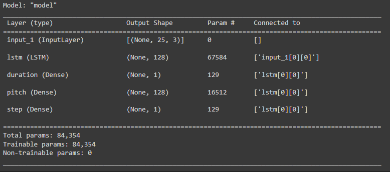
Let’s create the model.

inputs = tf.keras.Input((seq_length, 3))
x = tf.keras.layers.LSTM(128)(inputs)
outputs = {
  'pitch': tf.keras.layers.Dense(128, name='pitch')(x),
  'step': tf.keras.layers.Dense(1, name='step')(x),
  'duration': tf.keras.layers.Dense(1, name='duration')(x),
}
model = tf.keras.Model(inputs, outputs)
loss = {
      'pitch': tf.keras.losses.SparseCategoricalCrossentropy(
          from_logits=True),
      'step': mse,
      'duration': mse,
}
model.compile(loss=loss, optimizer=tf.keras.optimizers.Adam(learning_rate=0.5))
model.summary()

Output:

Let’s train the model.

callbacks = [
    tf.keras.callbacks.ModelCheckpoint(
        filepath='./training_checkpoints/ckpt_{epoch}',
        save_weights_only=True),
    tf.keras.callbacks.EarlyStopping(
        monitor='loss',
        patience=5,
        verbose=1,
        restore_best_weights=True),
]
history = model.fit(train_ds,epochs=epochs,callbacks=callbacks)

Output:

Now we are ready to use the model for the music generation. But before this, the predicted values from the model should be converted into the MIDI file.

Let’s make the prediction using the trained model.

def predict_next_note(notes: np.ndarray, keras_model: tf.keras.Model, temperature: float = 1.0) -> int:
  assert temperature > 0
  # Add batch dimension
  inputs = tf.expand_dims(notes, 0)
  predictions = model.predict(inputs)
  pitch_logits = predictions['pitch']
  step = predictions['step']
  duration = predictions['duration']
  pitch_logits /= temperature
  pitch = tf.random.categorical(pitch_logits, num_samples=1)
  pitch = tf.squeeze(pitch, axis=-1)
  duration = tf.squeeze(duration, axis=-1)
  step = tf.squeeze(step, axis=-1)
  # `step` and `duration` values should be non-negative
  step = tf.maximum(0, step)
  duration = tf.maximum(0, duration)
  return int(pitch), float(step), float(duration)

The above function is helping in making the predictions with the model. The below function will help in drawing the samples from the softmax distribution of notes instead of using the highest probability for sampling. 

temperature = 2.0
num_predictions = 120
sample_notes = np.stack([music_df[key] for key in key_order], axis=1)
# The initial sequence of notes; pitch is normalized similar to training
# sequences
input_notes = (
    sample_notes[:seq_length] / np.array([vocab_size, 1, 1]))
generated_notes = []
prev_start = 0
for _ in range(num_predictions):
  pitch, step, duration = predict_next_note(input_notes, model, temperature)
  start = prev_start + step
  end = start + duration
  input_note = (pitch, step, duration)
  generated_notes.append((*input_note, start, end))
  input_notes = np.delete(input_notes, 0, axis=0)
  input_notes = np.append(input_notes, np.expand_dims(input_note, 0), axis=0)
  prev_start = start
generated_notes = pd.DataFrame(
    generated_notes, columns=(*key_order, 'start', 'end'))
generated_notes.head(10)

Output:

Here we have the prediction from the model. Now we are required to make a function that can convert the data frame format into the MIDI format. Using the below-given function we can transform the predictions into MIDI. 

def df_to_midi(
  notes: pd.DataFrame,
  out_file: str, 
  instrument_name: str,
  velocity: int = 100,  # note loudness
) -> pretty_midi.PrettyMIDI:
  file = pretty_midi.PrettyMIDI()
  instrument = pretty_midi.Instrument(
      program=pretty_midi.instrument_name_to_program(
          instrument_name))
  prev_start = 0
  for i, note in notes.iterrows():
    start = float(prev_start + note['step'])
    end = float(start + note['duration'])
    note = pretty_midi.Note(
        velocity=velocity,
        pitch=int(note['pitch']),
        start=start,
        end=end,
    )
    instrument.notes.append(note)
    prev_start = start
  file.instruments.append(instrument)
  file.write(out_file)
  return file

generated = df_to_midi(
    music_df, out_file='generated.midi', instrument_name=instrument_name)

Here, the transformation of the data type has been done for confirmation. We can play the sound as we have done before.

waveform = generated.fluidsynth(fs=16000)
waveform_short = waveform[:30*16000]
display.Audio(waveform_short, rate=16000)

This is how we have got the generated music in a data file.

Final Words  

Here in the article, we have generated a music file using an RNN model. We trained this model on an older file. We can check the results where the pitch of the notes is different from the older file using the temperature parameter. We can control the randomness of the generated sample from the model. In this article, we just used a simple RNN model that can be improved more. I encourage users to try any other models also for automatic music generation.  

Reference

• Link to the above codes