Pruning as a concept was originally introduced to the field of deep learning by Yann LeCun in an eerie titled paper “Optimal Brain Damage”. The word pruning means trimming or cutting away the excess; in the context of machine learning and artificial intelligence, it involves removing the redundant or the least important parts of a model or search space. There can be multiple reasons for pruning a model:
- It can be used as a regularization technique to prevent overfitting
- A compression mechanism for creating smaller versions of models with marginal depreciation in model performance
- For reducing computational complexity and, in turn, inference time
Using Pruning to Regularize a Decision Tree Classifier
We’ll be training a DecisionTreeClassifier model on the Titanic dataset available on Kaggle. In this example, we’ll use pruning as a regularization technique for the overfitting-prone DecisionTreeClassifier.
- Fetch the dataset using the Kaggle API.
  import os
  from google.colab import drive
  drive.mount('/content/gdrive')
 os.environ['KAGGLE_CONFIG_DIR'] = "/content/gdrive/My Drive/Kaggle"
 # /content/gdrive/My Drive/Kaggle is the path where kaggle.json is present in the Google Drive
 %cd /content/gdrive/My Drive/Kaggle
 !kaggle competitions download -c titanic
- Load, clean, and split the data.
 data = pd.read_csv("train.csv")
 data = data.loc[:,("Survived","Pclass","Sex","Age","SibSp","Parch","Fare")]
 data.dropna(inplace=True)
 #'inplace=True' applies the code to the 'data' object.
 from sklearn.preprocessing import LabelEncoder
 le = LabelEncoder()
 data.Sex = le.fit_transform(data.Sex)
 x = data.iloc[:,1:]   # Second column until the last column
 y = data.iloc[:,0]    # First column (Survived) is our target
 from sklearn.model_selection import train_test_split
 #this function randomly split the data into train and test sets
 x_train, x_test, y_train, y_test = train_test_split(x, y, test_size=.3)
- Create a baseline model, train and evaluate it.
 from sklearn.tree import DecisionTreeClassifier
 dt_classifier = DecisionTreeClassifier()
 dt_classifier.fit(x_train, y_train)  #train parameters: features and target
 pred = dt_classifier.predict(x_test)
 from sklearn.metrics import accuracy_score
 accuracy_score(y_test, pred)

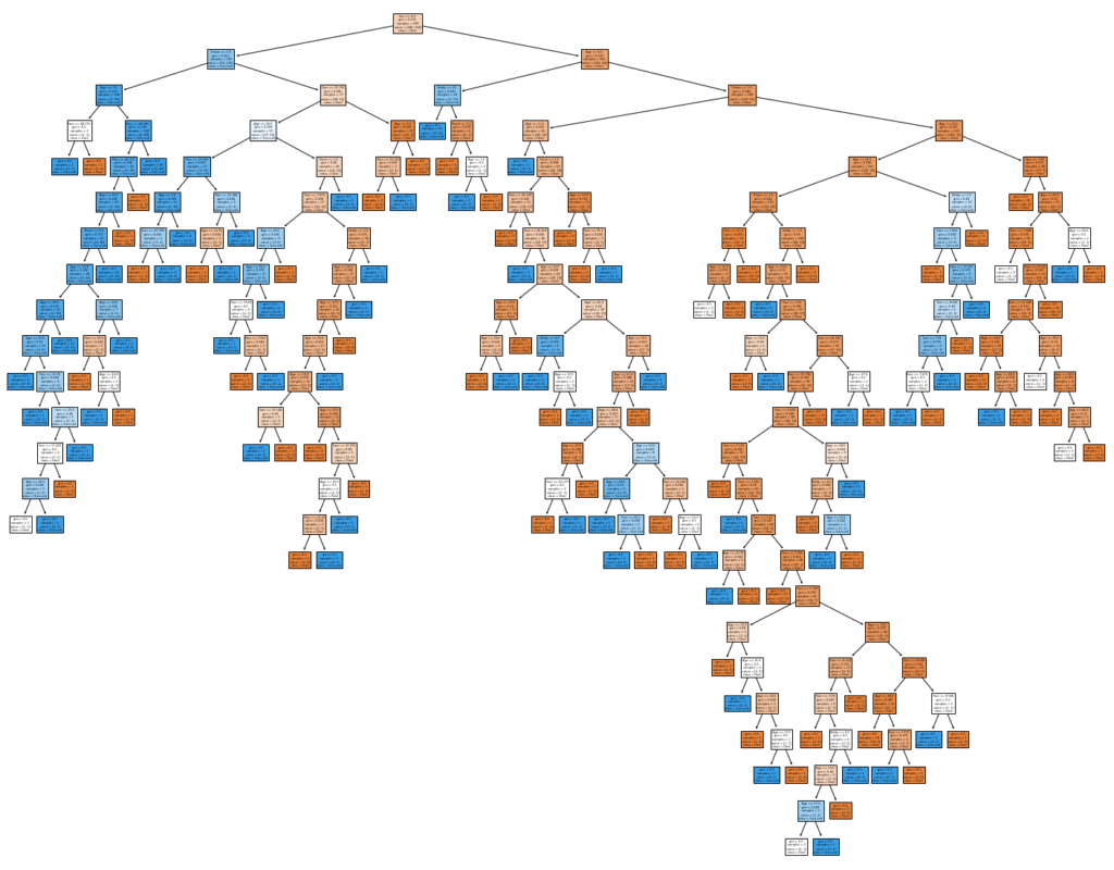
Let’s visualize the tree.
 fig = plt.figure(figsize=(25,20))
 _ = tree.plot_tree(dt_classifier,
                    feature_names=x.columns,
                    class_names=["Died", "Survived"],
                    filled=True)

- Prune the tree by searching for the optimum depth.
 acc = []
 for i in range(1,30):
  dt_classifier = DecisionTreeClassifier(max_depth=i)
  dt_classifier.fit(x_train, y_train)
  pred = dt_classifier.predict(x_test)
  acc.append(accuracy_score(y_test, pred))
 depth = acc.index(max(acc)) + 1
 dt_classifier = DecisionTreeClassifier( max_depth=depth)
 dt_classifier.fit(x_train, y_train)
 pred = dt_classifier.predict(x_test)
 accuracy_score(y_test, pred)

Let’s visualize the pruned tree.

We can see the huge difference in model complexity which is reflected in the increased model accuracy.
The Colab notebook for the above implementation can be found here.
Compressing a Neural Network
The following code has been taken from the official TensorFlow pruning example notebook available here. In this example, we illustrate the use of pruning for compressing a convolutional neural network model.
- Install tensorflow-model-optimization and create the baseline model
 ! pip install -q tensorflow-model-optimization
 import tempfile
 import os
 import tensorflow as tf
 import numpy as np
 from tensorflow import keras

 # Load MNIST dataset
 mnist = keras.datasets.mnist
 (train_images, train_labels), (test_images, test_labels) = mnist.load_data()

 # Normalize the input image so that each pixel value is between 0 to 1.
 train_images = train_images / 255.0
 test_images = test_images / 255.0

 # Define the model architecture.
 model = keras.Sequential([
   keras.layers.InputLayer(input_shape=(28, 28)),
   keras.layers.Reshape(target_shape=(28, 28, 1)),
   keras.layers.Conv2D(filters=12, kernel_size=(3, 3), activation='relu'),
   keras.layers.MaxPooling2D(pool_size=(2, 2)),
   keras.layers.Flatten(),
   keras.layers.Dense(10)
 ])

 # Train the classification model
 model.compile(optimizer='adam',
               loss=tf.keras.losses.SparseCategoricalCrossentropy(from_logits=True),
               metrics=['accuracy'])
 model.fit(
   train_images,
   train_labels,
   epochs=4,
   validation_split=0.1,
 )
- Evaluate and save the baseline model
 _, baseline_model_accuracy = model.evaluate(
     test_images, test_labels, verbose=0)
 print('Baseline test accuracy:', baseline_model_accuracy)
 _, keras_file = tempfile.mkstemp('.h5')
 tf.keras.models.save_model(model, keras_file, include_optimizer=False)
- Prune the neural network.
 import tensorflow_model_optimization as tfmot
 prune_low_magnitude = tfmot.sparsity.keras.prune_low_magnitude

 # Compute end step to finish pruning after 2 epochs.
 batch_size = 128
 epochs = 2
 validation_split = 0.1
 num_images = train_images.shape[0] * (1 - validation_split)
 end_step = np.ceil(num_images / batch_size).astype(np.int32) * epochs

 #Define model for pruning.
 pruning_params = {
 'pruning_schedule':
 tfmot.sparsity.keras.PolynomialDecay(initial_sparsity=0.50,
 final_sparsity=0.80,
 begin_step=0,
 end_step=end_step)
 }
 model_for_pruning = prune_low_magnitude(model, **pruning_params)

 # prune_low_magnitude requires a recompile.
 model_for_pruning.compile(optimizer='adam',
 loss=tf.keras.losses.SparseCategoricalCrossentropy(from_logits=True),
 metrics=['accuracy'])

 logdir = tempfile.mkdtemp()
 callbacks = [
 tfmot.sparsity.keras.UpdatePruningStep(),
 tfmot.sparsity.keras.PruningSummaries(log_dir=logdir),
 ]

 model_for_pruning.fit(train_images, train_labels,
 batch_size=batch_size, epochs=epochs,
 validation_split=validation_split,
 callbacks=callbacks)
- Evaluate and compare with baseline.
 _, model_for_pruning_accuracy = model_for_pruning.evaluate(
    test_images, test_labels, verbose=0)
 print('Baseline test accuracy:', baseline_model_accuracy)
 print('Pruned test accuracy:', model_for_pruning_accuracy)

There is a very small drop in performance, now let’s compare the size of the two models.
 def get_gzipped_model_size(file):
   # Returns size of gzipped model, in bytes.
   import os
   import zipfile
   _, zipped_file = tempfile.mkstemp('.zip')
   with zipfile.ZipFile(zipped_file, 'w', compression=zipfile.ZIP_DEFLATED) as f:
     f.write(file)
   return os.path.getsize(zipped_file)

 print("Size of gzipped baseline Keras model: %.2f bytes" % (get_gzipped_model_size(keras_file)))
 print("Size of gzipped pruned Keras model: %.2f bytes" % (get_gzipped_model_size(pruned_keras_file)))

Using pruning, we can create a 66% smaller model with a negligible drop in performance.
Using Alpha-Beta Pruning to Improve the Computational Efficiency of a Minimax AI
The minimax algorithm is used to choose the best-case scenario from all possible scenarios or a subset thereof. One of its more interesting use-cases is the AI opponent in turn-based games like tic-tac-toe, chess, connect4, etc. Simply put the minimax algorithm assigns “points” to different states of a game, i.e., the different stages a playing field such as the chessboard can take during a game. It assigns positive points to states that bring the AI closer to victory and negative points to states that bring the human player closer to victory. Based on the human moves, it stimulates the possible future moves and selects the one that adds the most points or deducts the least points.

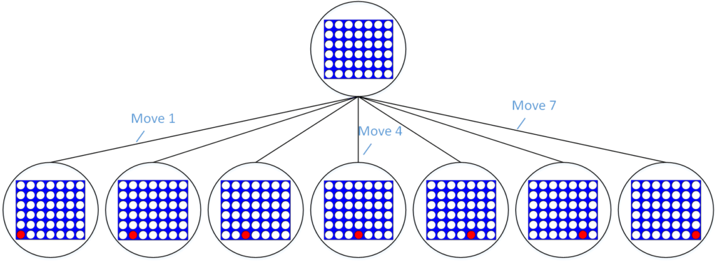
The state search tree grows exponentially; for example, the search tree for a connect4 AI grows as 7d, where d is the number of future turns the algorithm stimulates. This is computationally intensive and bogs down the minimax algorithm. Alpha-beta pruning is a search algorithm that reduces the number of states the minimax algorithm has to evaluate. It does this by removing nodes/branches that already have a better alternative; for instance, it would remove the branches that lead to checkmate if minimax has already evaluated a node/move that leads to the opponent losing several pieces.
I highly recommend this lecture for an in-depth understanding of the minimax algorithm and alpha-beta pruning.
The function that evaluates and scores board windows of size 4.
 def evaluate_window(window, piece):
     """ evaluates the four space wide window passed to it and returns appropriate score """
     score = 0
     opponent_piece = PLAYER_PIECE
     if piece == PLAYER_PIECE:
         opponent_piece = AI_PIECE
     if window.count(piece) == 4:
         score += 200
     elif window.count(piece) == 3 and window.count(EMPTY) == 1:
         score += 30
     elif window.count(piece) == 2 and window.count(EMPTY) == 2:
         score += 10
     if window.count(opponent_piece) == 3 and window.count(EMPTY) == 1:
         score -= 30
     return score
The function that creates horizontal, vertical and diagonal windows of size 4 and scores the possible board states.
 def board_score(board, piece):
     """ evaluates the passed (future) board for possible moves """
     score = 0
     # Scoring center column to add preference to play in the center
     center_list = [int(i) for i in list(board[:,COLUMNS//2])]
     center_count = center_list.count(piece)
     score += center_count * 20
     #Horizontal evaluation
     for r in range(ROWS):
         row_list = [int(i) for i in list(board[r,:])]
         for c in range(COLUMNS-3):
             four_window = row_list[c:c+4]
             score += evaluate_window(four_window, piece)
     #Vertical evaluation
     for c in range(COLUMNS):
         col_list = [int(i) for i in list(board[:,c])]
         for r in range(ROWS - 3):
             four_window = col_list[r:r+4]
             score += evaluate_window(four_window, piece)
     #Positively sloped diagonal evaluation
     for r in range(ROWS - 3):
         for c in range(COLUMNS-3):
             four_window = [board[r+i][c+i] for i in range(4)]
             score += evaluate_window(four_window, piece)
     #Negatively sloped diagonal evaluation
     for r in range(ROWS - 3):
         for c in range(COLUMNS-3):
             four_window = [board[r+(3-i)][c+i] for i in range(4)]
             score += evaluate_window(four_window, piece)
     return score
Minimax algorithm function.
 def minimax(board, depth, maximizingPlayer, alpha = -math.inf, beta = math.inf):
     is_terminal = is_terminal_node(board) #checks if the board is already full
     valid_locations = get_valid_locations(board) #gets columns that are not already full
     if depth == 0 or is_terminal: #base case for recursion
         if is_terminal:
             if winning(board, AI_PIECE):
                 return (100000000000000, None)
             elif winning(board, PLAYER_PIECE):
                 return (-100000000000000, None)
             else:
                 return (0, None)
         else:
             return (board_score(board, AI_PIECE), None)
     if maximizingPlayer:
         score = -math.inf
         column = random.choice(valid_locations)
         for col in valid_locations:
             row = get_next_open_row(board, col)
             #creating a copy so we don't modify the original game board
             board_copy = board.copy()
             drop_piece(board_copy, row, col, AI_PIECE)
             new_score =  minimax(board_copy, depth-1, False, alpha, beta)[0]
             if new_score > score:
                 score = new_score
                 column = col
             alpha = max(alpha, new_score)
             if alpha >= beta:
                 # print(alpha, beta)
                 break
         return new_score, column
     else:
         score = math.inf
         column = random.choice(valid_locations)
         for col in valid_locations:
             row = get_next_open_row(board, col)
             #creating a copy so we don't modify the original game board
             board_copy = board.copy()
             drop_piece(board_copy, row, col, PLAYER_PIECE)
             new_score = minimax(board_copy, depth-1, True, alpha, beta)[0]
             if new_score < score:
                 score = new_score
                 column = col
             beta = min(beta, new_score)
             if beta <= alpha:
                 # print(alpha, beta)
                 break
         return new_score, column
By introducing alpha-beta pruning, this AI can stimulate 6 moves into the future in real-time; this was limited to 4 before the optimization.
You can find the code for the connect4 game and minimax AI here.


